Unsupervised: Clustering Analysis
Unsupervised data mining: Clustering techniques
K-Means Clustering: This is a popular clustering algorithm that partitions data into k clusters based on the mean distance between data points and cluster centers. It aims to minimize the intra-cluster variance and is efficient for large datasets.
Application: Clustering Iris flowers in Iris dataset
Let’s first load the Iris dataset. This is a very famous dataset in almost all data mining, machine learning courses, and it has been an R build-in dataset. The dataset consists of 50 samples from each of three species of Iris flowers (Iris setosa, Iris virginicaand Iris versicolor). Four features(variables) were measured from each sample, they are the length and the width of sepal and petal, in centimeters. It is introduced by Sir Ronald Fisher in 1936 with 3 Iris Species.
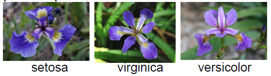
- Four features of flower: length and the width of sepal and petal
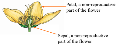
The iris flower data set is included in R. It is a data frame with 150 cases (rows) and 5 variables (columns) named Sepal.Length, Sepal.Width, Petal.Length, Petal.Width, and Species.
Ask Educate Us GPT
Why do we apply clustering analysis to the Iris dataset?
First, load iris data to the current workspace. This is a random grouping (first step).
data("iris")

# Scale the Iris dataset columns (excluding columns 2, 4, and 5)
iris1 <- scale(iris[,-c(2,4,5)])

# Get the number of rows in the scaled dataset
n <- nrow(iris1)

# Create a random index sample for splitting the dataset
index <- sample(2, n, replace = TRUE)

# Create two subsets based on the random index
iris.sub1 <- iris1[index == 1,]
iris.sub2 <- iris1[index == 2,]

# Calculate the mean of each column in the subsets
mean.sub1 <- apply(iris.sub1, 2, mean)
mean.sub2 <- apply(iris.sub2, 2, mean)

# Plot the scaled Iris dataset with different colors based on the subset index
plot(iris1, col = index + 1, pch = 16)

# Plot the mean of each subset as points in different colors
points(x = mean.sub1[1], y = mean.sub1[2], col = 2, pch = 8)
points(x = mean.sub2[1], y = mean.sub2[2], col = 3, pch = 8)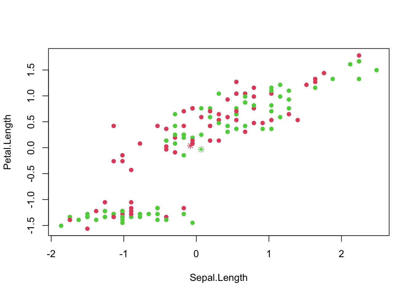
The next step
# Define a function 'Eudist' to calculate Euclidean distance between two vectors
Eudist <- function(x, y) sqrt(sum((x - y)^2))
# Calculate Euclidean distance between mean.sub1 and each row in iris1
d1 <- sapply(1:n, function(i) Eudist(mean.sub1, iris1[i,]))
# Calculate Euclidean distance between mean.sub2 and each row in iris1
d2 <- sapply(1:n, function(i) Eudist(mean.sub2, iris1[i,]))
# Determine the index of the minimum distance for each row to assign to a new index
index.new <- apply(cbind(d1, d2), 1, which.min)
# Create new subsets 'iris.sub1' and 'iris.sub2' based on the new index
iris.sub1 <- iris1[index.new == 1,]
iris.sub2 <- iris1[index.new == 2,]
# Calculate the mean of each column in the new subsets
mean.sub1 <- apply(iris.sub1, 2, mean)
mean.sub2 <- apply(iris.sub2, 2, mean)
# Create a scatter plot of iris1 with points colored based on the new index
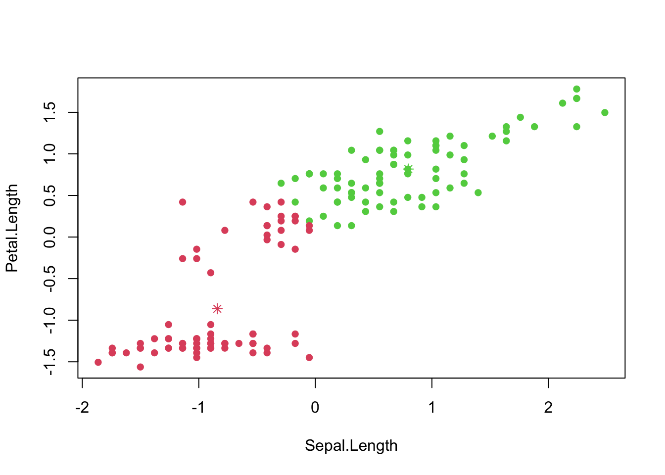
plot(iris1, col = index.new + 1, pch = 16)
# Plot the mean of each new subset as points in different colors on the scatter plot
points(x = mean.sub1[1], y = mean.sub1[2], col = 2, pch = 8)
points(x = mean.sub2[1], y = mean.sub2[2], col = 3, pch = 8)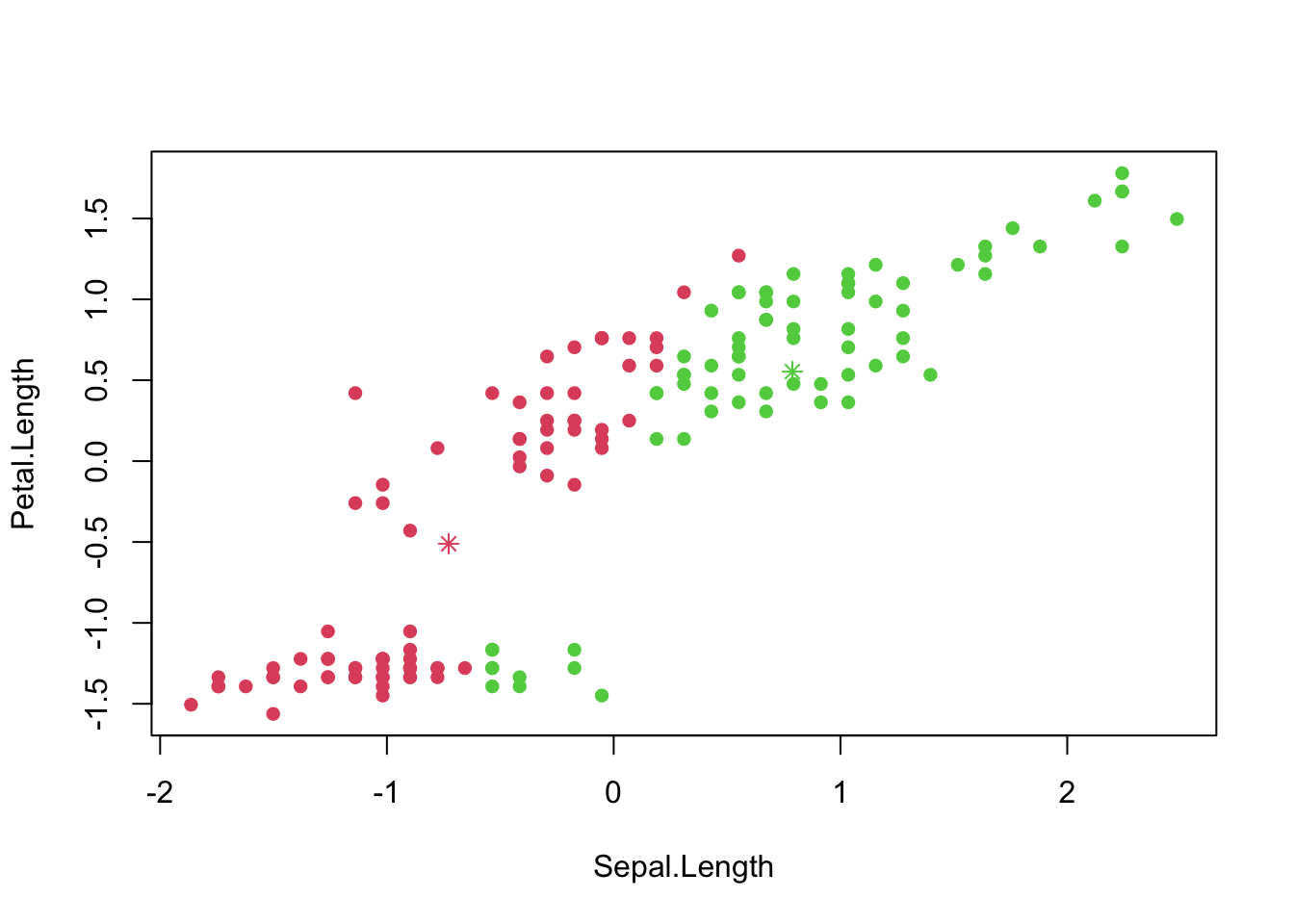
# Calculate the Euclidean distance between 'mean.sub1' and each row in 'iris1' and store in 'd1'
d1 <- sapply(1:n, function(i) Eudist(mean.sub1, iris1[i,]))

# Calculate the Euclidean distance between 'mean.sub2' and each row in 'iris1' and store in 'd2'
d2 <- sapply(1:n, function(i) Eudist(mean.sub2, iris1[i,]))

# Determine the index of the minimum distance between 'd1' and 'd2' for each row and assign to 'index.new'
index.new <- apply(cbind(d1, d2), 1, which.min)

# Create new subsets 'iris.sub1' and 'iris.sub2' based on 'index.new'
iris.sub1 <- iris1[index.new == 1,]
iris.sub2 <- iris1[index.new == 2,]

# Calculate the mean of each column in the new subsets
mean.sub1 <- apply(iris.sub1, 2, mean)
mean.sub2 <- apply(iris.sub2, 2, mean)

# Create a scatter plot of 'iris1' with points colored based on 'index.new'
plot(iris1, col = index.new + 1, pch = 16)

# Plot the mean of 'iris.sub1' as points in color 2 on the scatter plot
points(x = mean.sub1[1], y = mean.sub1[2], col = 2, pch = 8)

# Plot the mean of 'iris.sub2' as points in color 3 on the scatter plot
points(x = mean.sub2[1], y = mean.sub2[2], col = 3, pch = 8)